Monopolies
The most important lesson to remember with monopolies is that monopolist firms will underproduce and overcharge—Q will be lower and P will be higher than what should happen if the market is in equilibrium.
As with profit maximization and supply and demand, there are a ton of other resources online that you can references for additional help. Khan Academy’s monopoly unit is especially useful and easy to follow.
In this example, let’s assume that the demand for some product is:
\[ D: P = -Q + 40 \]
A single firm that is a monopolist has the following total cost function:
\[ TC: P = Q^2 + 140 \]
Using calculus, we can find the marginal cost function by taking the first derivative:
\[ MC: P = 2Q \]
If this firm isn’t a monopolist, and the marginal cost here represented the supply of the whole market, we’d have this market equilibrium:
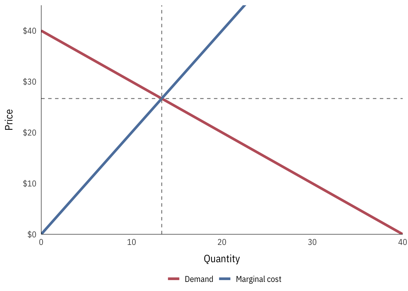
At this equilibrium, the best quantity is 13.33, and the best price is $26.67.
However, because this firm is a monopolist, it doesn’t have to take the prevailing price out in society. Instead, it can set the price to whatever maximizes its own profit. The formula for maximizing profit is \(MR = MC\), which means we need to find the formula for both marginal revenue and marginal cost. We already know the formula for marginal cost—that’s the blue line in the graph above:
\[ MC: P = 2Q \]
We don’t have the formula for marginal revenue, but we can figure it out with some tricky algebra moves. Remember that the general formula for total revenue is \(TR = PQ\), or the price × the quantity of stuff sold. We already know the price of things demanded—that’s the demand curve. If we substitute the demand curve formula into the TR formula in place of P, we can find the formula for total revenue:
\[ \begin{aligned} TR &= PQ \\ &= (-Q + 40)Q \\ &= -Q^2 + 40Q \end{aligned} \]
Total revenue is thus \(Q^2 + 40Q\). If we find the first derivative of that, we’ll have the marginal revenue:
\[ MR = -2Q + 40 \]
Phew. Now we have equations for marginal cost and for marginal revenue, so we can set them equal to each other and find where they cross using algebra:
\[ \begin{aligned} MR &= MC \\ -2Q + 40 &= 2Q \\ 40 &= 4Q \\ 10 &= Q \end{aligned} \]
The ideal quantity to maximize profits is thus 10. We can see this in a graph, along with the ideal price (this is point B):
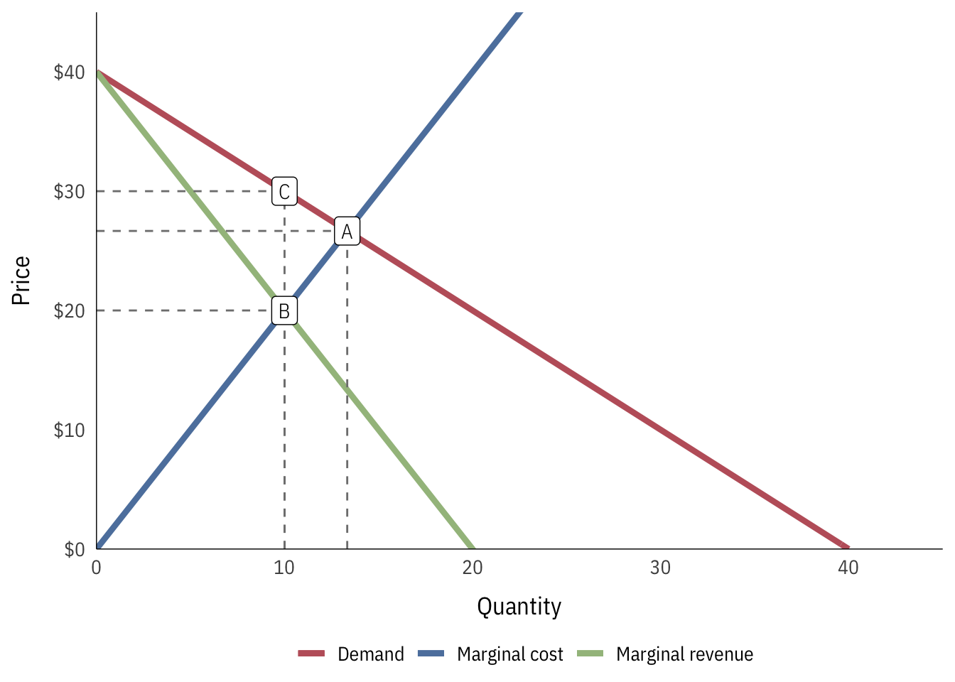
We can see that there’s a reduction in quantity. They should be producing 13.33 units, but now they’re only making 10. The price for this new lower quantity is lower too, but there’s now a problem! Based on the demand curve, society is willing to pay up to $30 per product, since only 10 are being made. This means that even though the firm should only charge $20, given where MC and MR cross, it can raise the price and charge $30 instead, leading to point C. Now there are fewer products being produced and they’re more expensive!
This sequence of events creates the monopoly triangle:
- According to supply and demand, the firm should produce and sell at point A
- Because they have market power and are a monopoly, the firm can produce where its marginal revenue = its marginal costs, meaning it should produce at point B
- Point B leads to a lower Q, and society is willing to pay a higher price for that lower quantity, so the firm will raise the price to point C, thus underproducing and overcharging.
This monopoly has a few different consequences beyond lower quantities and higher prices:
- Deadweight loss is created
- Producer surplus grows
- Consumer surplus shrinks
We can calculate these exact values by using geometry to find the areas of these different rectangles and triangles:
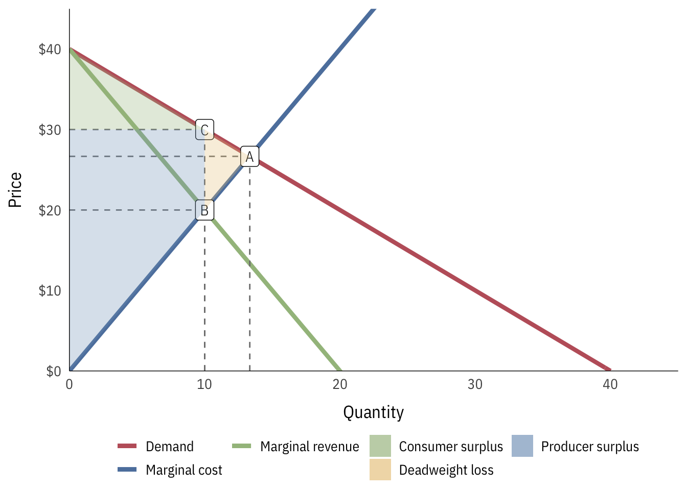
- Deadweight loss: \(1/2 \times (13.333-10) \times (30 - 20) = \$16.67\)
- Consumer surplus: \(1/2 \times 10 \times 10 = \$50\)
- Producer surplus:
- Triangle part: \(1/2 \times 10 \times 20 = \$100\)
- Rectangle part: \(10 \times 10 = \$100\)
- Total: \(\$200\)